How quick and big would a software intelligence explosion be?
By Tom_Davidson, TomHoulden, Forethought @ 2025-08-05T15:47 (+14)
AI systems may soon fully automate AI R&D. Myself and Daniel Eth have argued that this could precipitate a software intelligence explosion – a period of rapid AI progress due to AI improving AI algorithms and data.
But we never addressed a crucial question: how big would a software intelligence explosion be?
This new paper fills that gap.
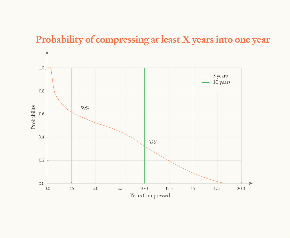
Overall, we guess that the software intelligence explosion will probably (~60%) compress >3 years of AI progress into <1 year, but is somewhat unlikely (~20%) to compress >10 years into <1 year. That’s >3 years of total AI progress at recent rates (from both compute and software), achieved solely through software improvements. If compute is still increasing during this time, as seems likely, that will drive additional progress.
The existing discussion on the “intelligence explosion” has generally split into those who are highly sceptical of intelligence explosion dynamics and those who anticipate extremely rapid and sustained capabilities increases. Our analysis suggests an intermediate view: the software intelligence explosion will be a significant additional acceleration at just the time when AI systems are surpassing top humans in broad areas of science and engineering.
Like all analyses of this topic, this paper is necessarily speculative. We draw on evidence where we can, but the results are significantly influenced by guesswork and subjective judgement.
Summary
How the model works
We use the term ASARA to refer to AI that can fully automate AI research (ASARA = “AI Systems for AI R&D Automation”). For concreteness, we define ASARA as AI that can replace every human researcher at an AI company with 30 equally capable AI systems each thinking 30X human speed.
We simulate AI progress after the deployment of ASARA.
We assume that half of recent AI progress comes from using more compute in AI development and the other half comes from improved software. (“Software” here refers to AI algorithms, data, fine-tuning, scaffolding, inference-time techniques like o1 — all the sources of AI progress other than additional compute.) We assume compute is constant and only simulate software progress.
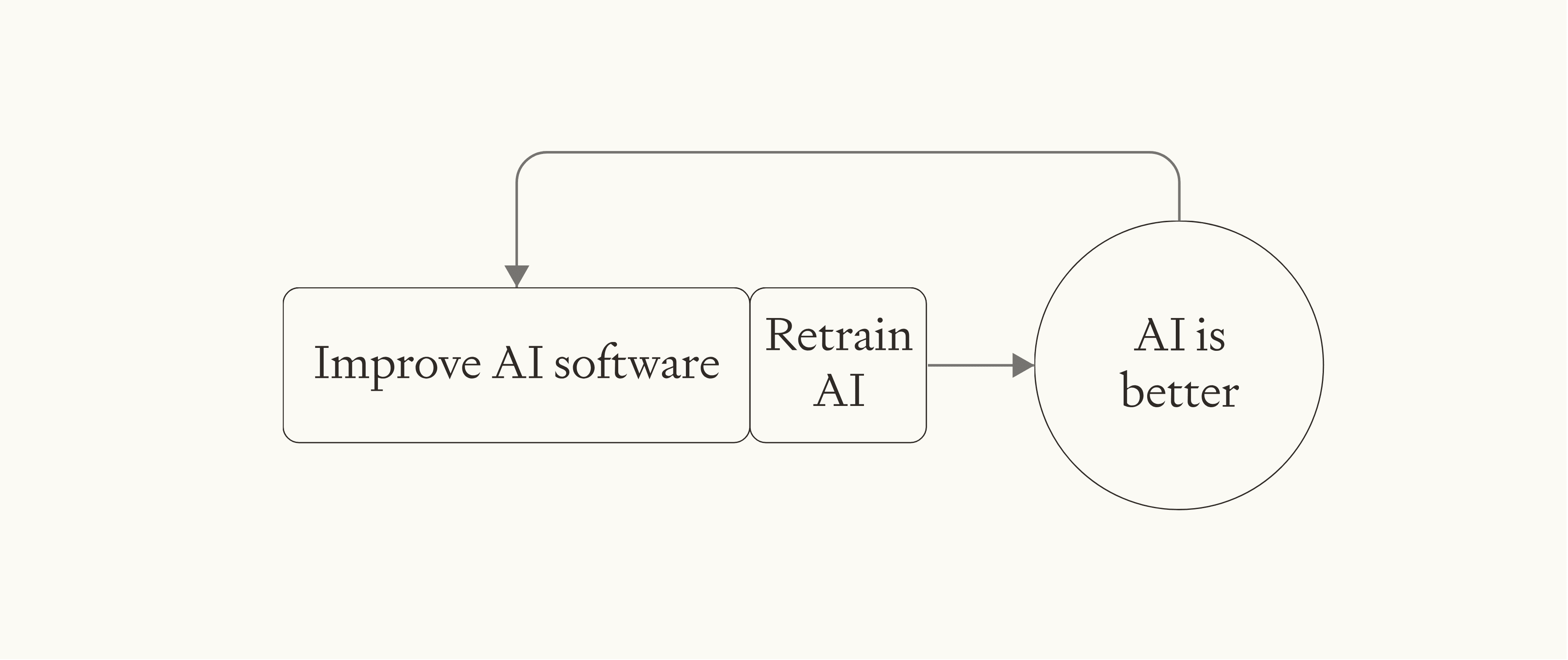
We assume that software progress is driven by two inputs: 1) cognitive labour for designing better AI algorithms, and 2) compute for experiments to test new algorithms. Compute for experiments is assumed to be constant. Cognitive labour is proportional to the level of software, reflecting the fact AI has automated AI research.
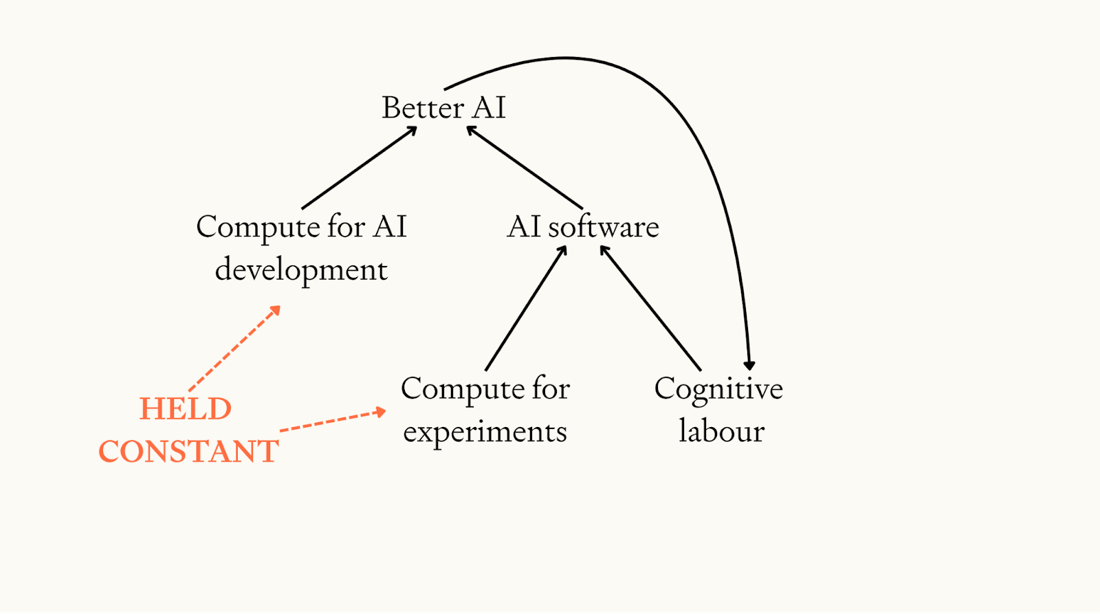
So the feedback loop we simulate is: better AI → more cognitive labour for AI research → more AI software progress → better AI →…
The model has three key parameters that drive the results:
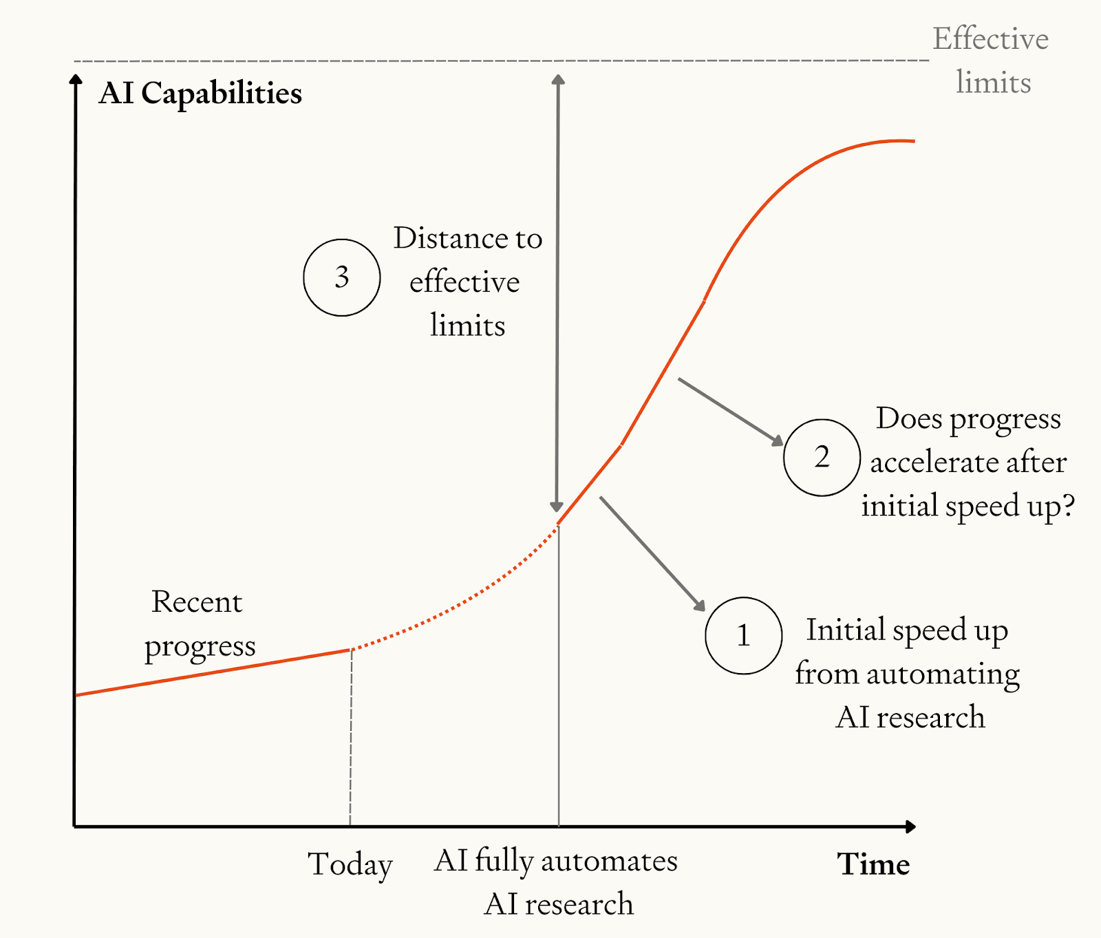
- Initial speed-up. When ASARA is initially deployed, how much faster is software progress compared to the recent pace of software progress?
- Returns to software R&D. After the initial speed-up from ASARA, does the pace of progress accelerate or decelerate as AI progress feeds back on itself?
- This is given by the parameter . Progress accelerates if and only if .
- depends on 1) the extent to which software improvements get harder to find as the low hanging fruit are plucked, and 2) the strength of the “stepping on toes effect” whereby there are diminishing returns to more researchers working in parallel.
- Distance to “effective limits” on software. How much can software improve after ASARA before we reach fundamental limits to the compute efficiency of AI software?
- The model assumes that, as software approaches effective limits, the returns to software R&D become less favourable and so AI progress decelerates.
The following table summarises our estimates of the three key parameters:
| Parameter | Estimation methods | Values used in the model |
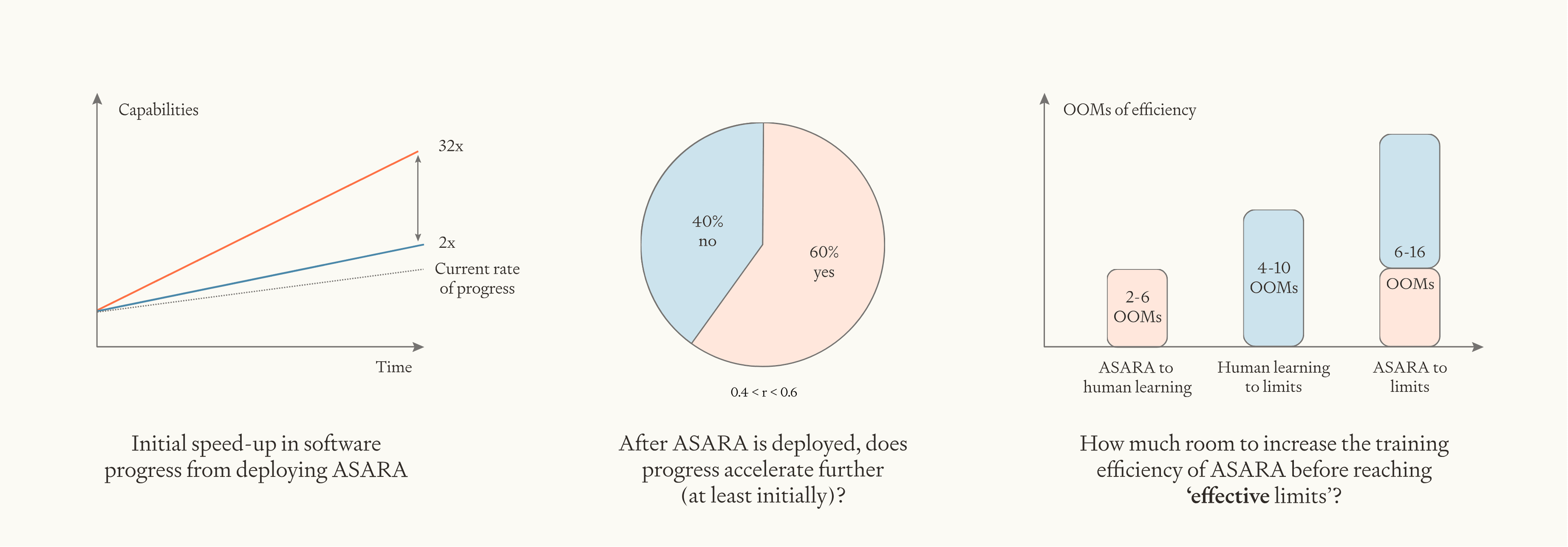
| Initial speed-up in software progress from deploying ASARA |
| Compared to progress in 2020-2024, software progress will be faster by a factor of 2 - 32, with a median of 8 |
Returns to software R&D
(After the initial speed-up, does progress accelerate or decelerate?)
|
| The pace of software progress will probably (~60%) accelerate over time after the initial speed-up (at least initially).
(We estimate 0.4 < r < 3.6, with a median of r = 1.2) |
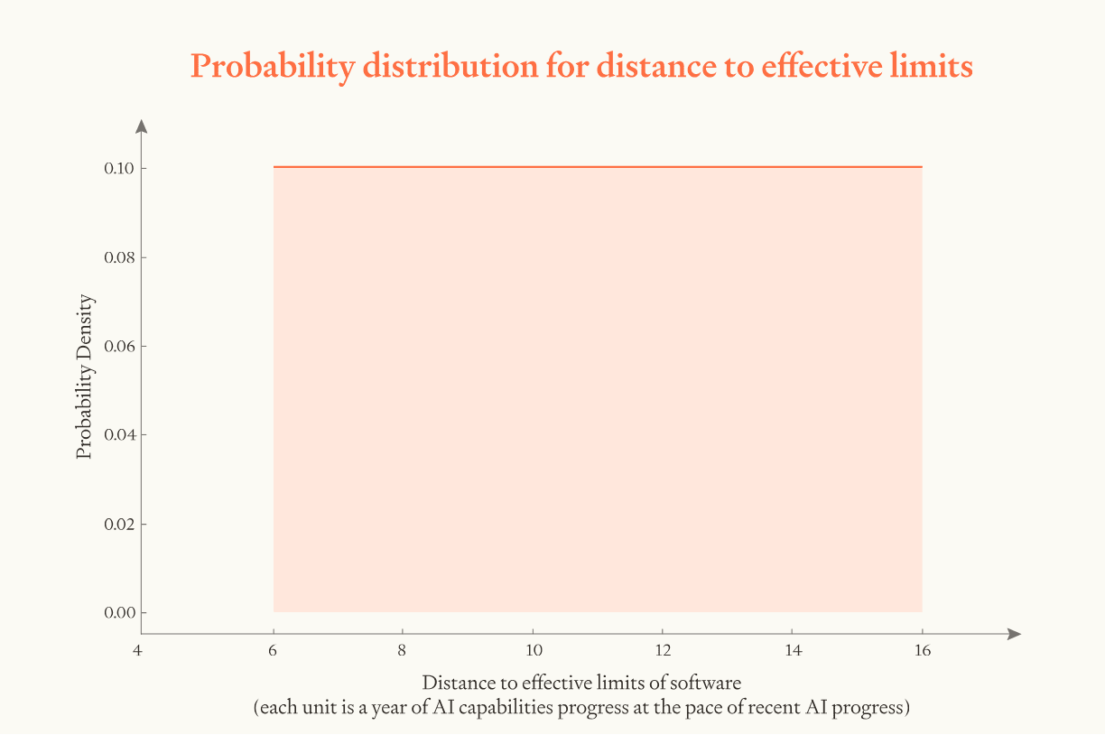
| Distance to “effective limits” of AI software |
| 6 - 16 OOMs of efficiency gains after ASARA before hitting effective limits
This translates to 6-16 years worth of AI progress, because the effective compute for AI training has recently risen by ~10X/year |
We put log-uniform probability distributions over the model parameters and run a Monte Carlo (more).
You can enter your own inputs to the model on this website.
Results
Here are the model’s bottom lines (to 1 sig fig):
| Years of progress | Compressed into ≤1 year | Compressed into ≤4 months |
| ≥3 years | ~60% | ~40% |
| ≥10 years | ~20% | ~10% |

Remember, the simulations conservatively assume that compute is held constant. They compare the pace of AI software progress after ASARA to the recent pace of overall AI progress, so “3 years of progress in 1 year” means “6 years of software progress in 1 year”.
While the exact numbers here are obviously not to be trusted, we find the following high-level takeaway meaningful: averaged over one year, AI progress could easily be >3X faster, could potentially be >10X faster, but won’t be 30X faster absent a major paradigm shift. In particular:
- Initial speed-ups of >3X are likely, and the returns to software R&D are likely high enough to prevent progress slowing back down before there is 3 years of progress.
- If effective limits are >10 OOMs away and returns to software R&D remain favourable until we are close to those limits, progress can accelerate for long enough to get ten years of progress in a year. We think it’s plausible but unlikely that both these conditions hold.
- To get 30 years of progress in one year, either you need extremely large efficiency gains on top of ASARA (30 OOMs!) or a major paradigm shift that enables massive progress without significant increases in effective compute (which seems more likely).
We also consider two model variants, and find that this high-level takeaway holds in both:
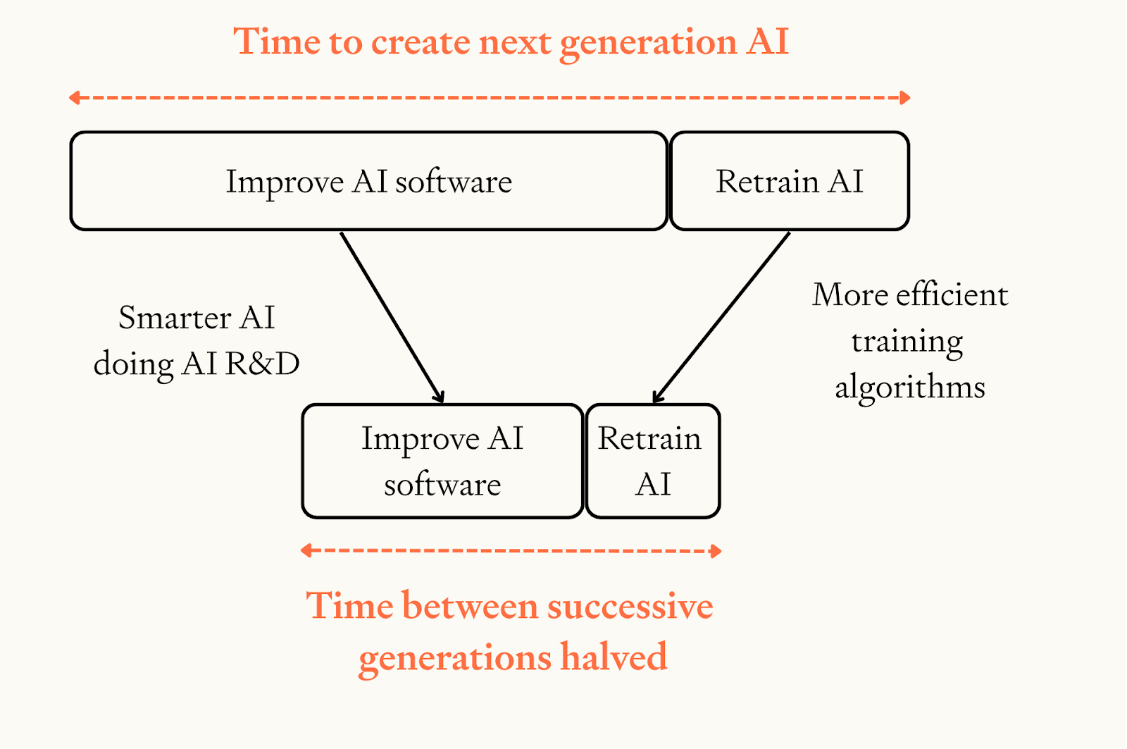
- Retraining new models from scratch. In this variant, some fraction of software progress is “spent” making training runs faster as AI progress accelerates. More.
- Gradual boost. In this variant, we simulate a gradual increase in AI capabilities from today’s AI to ASARA, with software progress accelerating along the way. More.
Discussion
If this analysis is right in broad strokes, how dramatic would the software intelligence explosion be?
There’s two reference points we can take.
One reference point is historical AI progress. It took three years to go from GPT-2 to ChatGPT (i.e. GPT-3.5); it took another three years to go from GPT-3.5 to o3. That’s a lot of progress to see in one year just from software. We’ll be starting from systems that match top human experts in all parts of AI R&D, so we will end up with AI that is significantly superhuman in many broad domains.
Another reference point is effective compute. The amount of effective compute used for AI development has increased at roughly 10X/year. So, three years of progress would be a 1000X increase in effective compute; six years would be a million-fold increase. Ryan Greenblatt estimates that a million-fold increase might correspond to having 1000X more copies that think 4X faster and are significantly more capable. In which case, the software intelligence explosion could take us from 30,000 top-expert-level AIs each thinking 30X human speed to 30 million superintelligent AI researchers each thinking 120X human speed, with the capability gap between each superintelligent AI researcher and the top human expert about 3X as big as the gap between the top expert and a median expert.[1][2]
Limitations
Our model is extremely basic and has many limitations, including:
- Assuming AI progress follows smooth trends. We don’t model the possibility that superhuman AI unlocks qualitatively new forms of progress that amount to a radical paradigm shift; nor the possibility that the current paradigm stops yielding further progress shortly after ASARA. So we’ll underestimate the size of the tails in both directions.
- No gears-level analysis. We don’t model how AIs will improve software in a gears-level way at all (e.g. via generating synthetic data vs by designing new algorithms). So the model doesn’t give us insight into these dynamics. Instead, we extrapolate high-level trends about how much research effort is needed to double the efficiency of AI algorithms. And we don’t model specific capabilities, just the amount of “effective training compute”.
- “Garbage in, garbage out”. We’ve done our best to estimate the model parameters, but there are massive uncertainties in all of them. This flows right through to the results.
- This uncertainty is especially large for the “distance to effective limits” parameter.
- You can choose your own inputs to the model here!
- No compute growth. The simulation assumes that compute doesn’t grow at all after ASARA is deployed, which is obviously a conservative assumption.
Overall, we think of this model as a back-of-the-envelope calculation. It’s our best guess, and we think there are some meaningful takeaways, but we don’t put much faith in the specific numbers.
Structure of the paper
The rest of the paper lays out our analysis in more detail. We proceed as follows:
- We explain how this paper relates to previous work on the intelligence explosion.
- We clarify the scenario being considered.
- We outline the model dynamics in detail.
- We evaluate which parameters values to use – this is the longest section.
- We summarise the parameter values chosen.
- We describe the model predictions.
- We discuss limitations.
Relation to previous work
Eth & Davidson (2025) argue that a software intelligence explosion is plausible. They focus on estimating the returns to software R&D and argue they could allow for accelerating AI progress after ASARA is deployed. This paper builds on this work by doing more detailed quantitative modelling of the software intelligence explosion, especially the initial speed-up in progress due to ASARA and the distance to the effective limits of software. Both Eth and Davidson (2025) and this paper draw heavily on estimates from Besiroglu et al. (2024).
Davidson (2023) (and its online tool) and Davidson et al. (2025) model all inputs to AI progress including hardware R&D and increased compute spending. Davidson (2023) also models the effects of partial automation. By contrast, this paper (and its own online tool) more carefully models the dynamics of software progress after full automation.
Kokotajlo & Lifland (2025) is the research supplement for AI-2027. They use a different methodology to forecast a software intelligence explosion, relying less on estimates of the returns to software R&D and more on estimates for how long it would take human researchers to develop superhuman AI without AI assistance. Their forecast is towards the more aggressive end of our range. A rough calculation suggests that our model assigns a ~20% probability to the intelligence explosion being faster than their median scenario.[3]
Erdil & Barnett (2025) express scepticism about an software intelligence explosion lasting for more than one order of magnitude of algorithmic progress. By contrast, this paper predicts it will likely last for at least several orders of magnitude.
Bostrom (2014) is uncertain about the speed from human-level to superintelligent AI, but finds transitions of days or weeks plausible. By contrast, this paper’s forecasts are more conservative.
Yudkowsky (2013) argues that there will be an intelligence explosion that lasts “months or years, or days or seconds”. It draws upon wide-ranging evidence from chess algorithms, human evolution, and economic growth. By contrast our paper focuses on recent evidence from modern machine learning.
Scenario
We analyse a scenario in which:
- ASARA is deployed internally within an AI developer to fully automate AI R&D.
- There are no further human bottlenecks on the pace of progress – i.e. no pauses to help humans understand developments, ensure AI is developed safely, or assess legal risk.
- After ASARA is deployed, the compute used for AI R&D remains constant over time.
- Recent scaling laws on capabilities roughly continue: each doubling of effective compute for developing AI improves capabilities by the same amount as it has in recent years.
We forecast software progress after ASARA is deployed (though a variant also simulates a gradual ramp-up to ASARA).
Model dynamics
(Readers can skip this section and go straight to the estimates of the parameter values.)
The model simulates the evolution of AI software.
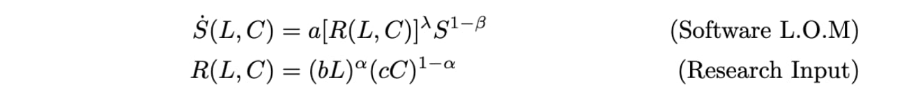
We start with the following standard semi-endogenous law of motion for AI software:
where:
- is the level of AI software
- is the cognitive labour used for improving software
- is compute for experiments, assumed to be constant
- captures “stepping on toes”, whereby there are diminishing returns to applying more research effort in parallel (nine women can’t make a baby in a month!).
- captures software improvements getting harder to find as software improves
- captures the diminishing returns of cognitive labour to improving software
- , , and are constants that are collectively pinned down by growth rates at the beginning of the model
Note that this model assumes that, in software R&D, the elasticity of substitution between cognitive labour and compute equals 1. This is an important assumption, discussed further here and here.
From these equations we derive how much faster (or slower) each successive doubling of software is compared to the last:
To reduce the number of distinct parameters and use parameters that can be directly estimated from the empirical evidence we have, we write this as:
where and are deflated stepping on toes and returns to software R&D; deflated by the diminishing returns of cognitive labour as a research input, . Specifically,
Notice the doubling time becomes smaller just if .
The standard semi-endogenous growth model allows growth to proceed indefinitely. If , that means software tends to infinity in finite time.[4] But in reality, there will be some effective limit on how good software can become. To model this, we define a ceiling for software and assume declines as software approaches the ceiling – specifically, each time software doubles we subtract some constant from . We choose so that, once software reaches the ceiling, and further progress in software is impossible. (The way we’ve modelled the change in is very specific; it could be too aggressive or too conservative – see more.)
Pseudocode
This leaves us with the following pseudocode:
The pseudo-code requires four inputs:
- . We calculate this from 1) the recent software doubling time (which we assume is 3 months) and 2) our estimate of the initial speed-up of software progress from deploying ASARA.
- , i.e. the distance to the effective limits on software.[5]
- , the (deflated) returns to software R&D when ASARA is first developed.
- , the diminishing returns to parallel labour.
The four bolded quantities – initial speed-up, distance to effective limits, returns to software R&D, and diminishing returns to parallel labour – are the four parameters that users of the model must specify. We estimate them in the next section.
To translate the model’s trajectories of software progress into units of overall AI progress, the model assumes that software progress has recently been responsible for 50% of total AI progress.
You can choose your own inputs to the model here; code for the simulations produced is here.
Parameter values
This section estimates the four main parameters of the model:
- Initial speed-up of software progress from deploying ASARA
- Returns to software R&D
- Distance to effective limits of software
- Diminishing returns to parallel labour (less important)
Initial speed-up of software progress from deploying ASARA
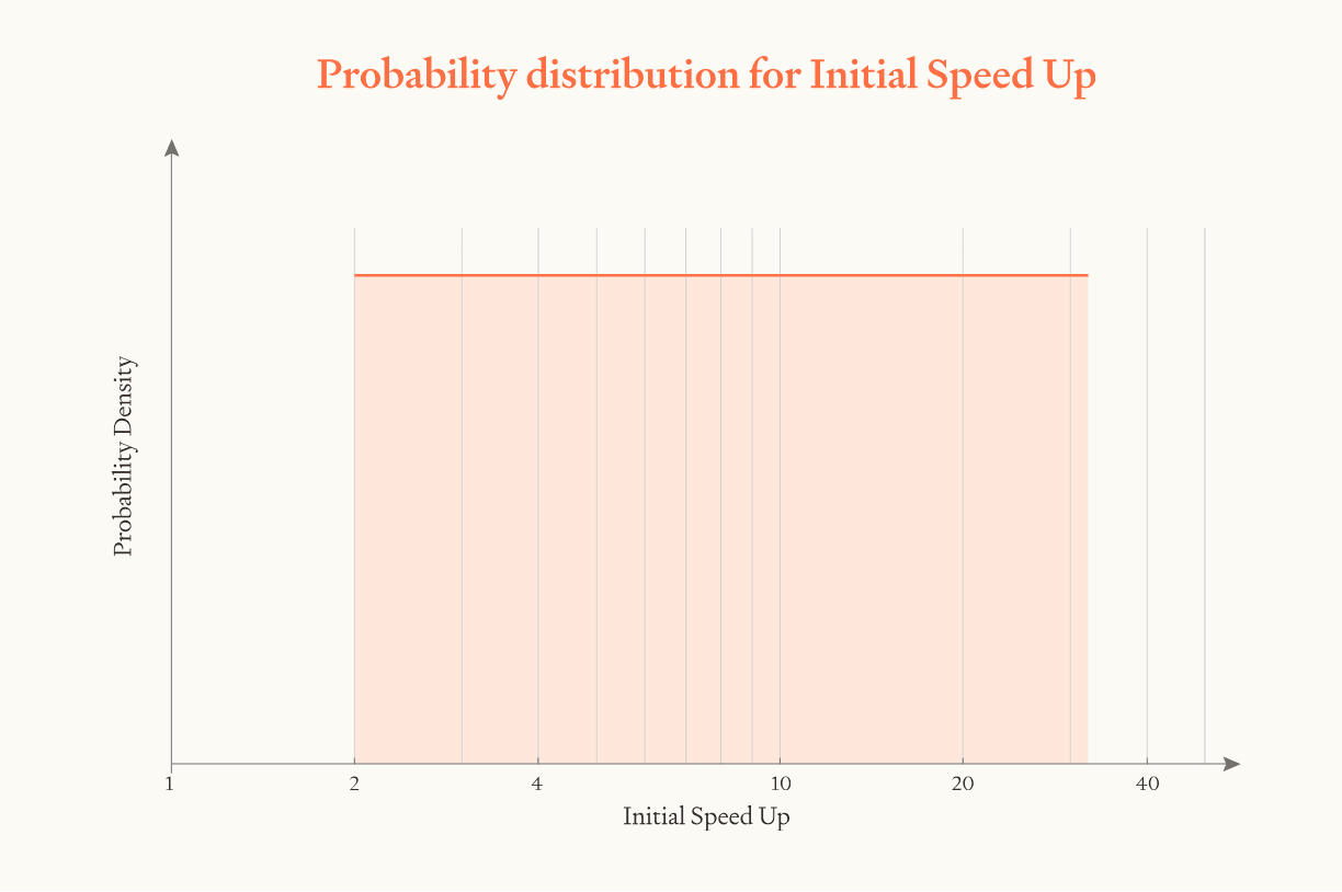
After ASARA is deployed, software progress is faster by a factor of . is sampled from a log-uniform distribution between 2 and 32, median 8.
ASARA is a vague term – it just refers to full automation of AI R&D. But you could automate AI R&D by replacing each human with a slightly-better AI system, or by replacing them with 1 million way-better AI systems. In the former case the amount of cognitive labour going into AI R&D wouldn’t increase much, in the latter case it would increase by a huge factor.
So what definition of ASARA should we use? There’s a few considerations here (see more in footnote[6]), but the most important thing is to pick one definition and stick with it. Let’s stipulate that ASARA can replace each human researcher with 30 equally capable AI systems each thinking 30X human speed.[7] So the total cognitive labour for AI R&D increases by 900X.
ASARA (so defined) is less capable than AI 2027’s superhuman AI researcher, which would be equally numerous and fast as ASARA but replace the capabilities of the best human researcher (which we expect to be worth much more than 30 average human researchers). ASARA is probably closer to AI 2027’s superhuman coder, that matches top humans at coding but lags behind on research taste.
How much faster would ASARA, so defined, speed up software progress compared to the recent pace of software progress?
There are a few angles on this question:
- Survey researchers about speed-ups from abundant cognitive labour. This paper surveyed five researchers about how much ASARA would speed up the pace of AI progress. They used the same definition of ASARA as we’re using.
- When asked outright about the total speed-up, responses varied from 2X to 20X with a geometric mean of 5X. If software progress accounts for 50% of total progress, then the corresponding speed-up in software progress is 10X.
- When asked to estimate the speed-ups from different sources separately (e.g. reducing bugs, doing experiments at small scales), their estimates were higher, with a geometric mean of 14X. This translates into a speed-up in software progress of 28X.
- Survey researchers about the per-person slowdown from reduced compute. If you have way more virtual researchers, each one of them will have much less compute. How much more slowly will they make progress?
- Analysing specific sources of speed-up. AI 2027 evaluates specific speed-ups that abundant AI labour would enable — smaller experiments, better prioritisation, better experiments, less wasted compute. They explicitly account for compute bottlenecks in their analysis but still find large gains.
- Thought experiment about an AI lab with fewer + slower researchers. ASARA would increase the number and speed of researchers working on AI R&D. We might expect the opposite effect if we instead decreased the number of human researchers and made them much slower. In particular, imagine if frontier AI labs had 30X fewer researchers and they each thought 30X more slowly – how much slower would AI progress be? If you think progress would be a lot slower, that suggests ASARA might speed up progress a lot. Ryan Greenblatt and Eli LIfland explore this idea here.
- Use a simple economic model of R&D (the same model as we use in our simulation)
- In particular, this model is:
- Our median model assumptions correspond to , .
- ASARA brings two changes: 1) 30X as many researchers in parallel, 2) every researcher thinks 30X faster
- 1) multiplies by 30, which multiplies the rate of software progress by .
- 2) multiplies by 30 which multiplies the rate of software progress by .
- Multiplying these independent effects together, we get the total speed up of 15X.
| Method | Forecasted initial speed-up in software progress due to ASARA |
| Survey researchers about speed-ups from abundant cognitive labour – ask directly about total gain | 10X |
| Survey researchers about speed-ups from abundant cognitive labour – ask separately about different sources of speed-up | 28X |
| Survey researchers about the per-person slowdown from reduced compute | 21X |
| AI 2027 analysis of specific sources of speed-up | 5X for superhuman coder (less capable than ASARA) 417X from superhuman AI researcher (more capable than ASARA) |
| Thought experiment about a lab with fewer and slower researchers | Big multiplier (no specific number suggested) |
| Use a simple economic model of R&D | 15X |
These methods may be too aggressive. Before we have ASARA, less capable AI systems may still accelerate software progress by a more moderate amount, plucking the low-hanging fruit. As a result, ASARA has less impact than we might naively have anticipated.
Overall, we're going to err conservative here and use a log-uniform distribution between 2 and 32, centred on 8. In other words, deploying ASARA would speed up progress by some factor; our upper bound for this factor is 32; our lower bound is 2; our median is 8.
As we've said, there’s massive uncertainty here and significant room for reasonable disagreement.
To visualise how this parameter affects the results, we can run simulations with the initial speed up equalling 2, 8, and 32:
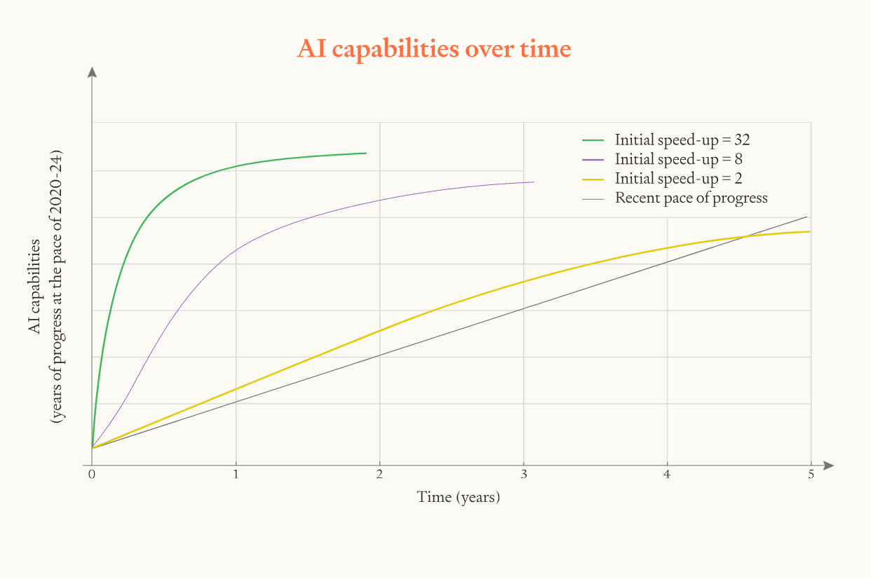
In the model, if the initial speed is twice as fast then the whole software intelligence explosion happens twice as fast and the maximum pace of progress is twice as fast.
Returns to software R&D, r
On our median guess for returns to software R&D, progress initially gets faster over time but then starts slowing down after training efficiency improves by a few OOMs.
After the initial speed-up from deploying ASARA, will software progress become faster or slower over time?
This depends on the model parameter .
If , then software progress will slow down over time. If , software progress will remain at the same exponential rate. If , software progress will speed up over time. (See Eth & Davidson (2025) for explanation.)
Luckily, the value of can be studied empirically. is the answer to the following question:
When (cumulative[9]) cognitive research inputs double, how many times does software double[10]?
We can study this question by observing how many times software has doubled each time the human researcher population has doubled.
What does it mean for “software” to double? A simple way of thinking about this is that software doubles when you can run twice as many parallel copies of your AI with the same compute. But software improvements don’t just improve runtime efficiency: they also improve capabilities and thinking speed. We translate such improvements to an equivalent increase in parallel copies. So if some capability improvement c increases the pace of AI progress by the same amount as doubling the number of parallel copies, we say that c doubled software. In practice, this means we’ll need to make some speculative assumptions about how to translate capability improvements into an equivalently-useful increase in parallel copies. For an analysis which considers only runtime efficiency improvements, see this appendix. |
Box 1: What does it mean for “software” to double?
The best quality data on this question is Epoch’s analysis of computer vision training efficiency. They estimate : every time the researcher population doubled, training efficiency doubled 1.4 times.[11] We can use this as a starting point, and then make various adjustments:
- Upwards for improving capabilities. Improving training efficiency improves capabilities, as you can train a model with more effective compute. Imagine we use a 2X training efficiency gain to train a model with twice as much effective compute. How many times would that double “software”? (I.e., how many doublings of parallel copies would be equally useful?) There are various sources of evidence here:[12] toy ML experiments suggest the answer is ~1.7; human productivity studies suggest the answer is ~2.5. We put more weight on the former, so we'll estimate 2. This doubles our median estimate to .
- Upwards for post-training enhancements. So far, we’ve only considered pre-training improvements. But post-training enhancements like fine-tuning, scaffolding, and prompting also improve capabilities (o1 was developed using such techniques!). These can allow faster thinking, which could be a big factor. But there might also be strong diminishing returns to post-training enhancements holding base models fixed. We'll adjust our median estimate up from 2.8 to .
- Downwards for less growth in compute for experiments. Today, rising compute means we can run increasing numbers of GPT-3-sized experiments each year. This helps drive software progress. But compute isn’t growing in our scenario. That might mean that returns to additional cognitive labour diminish more steeply. On the other hand, the most important experiments are ones that use similar amounts of compute to training a SOTA model. Rising compute hasn't actually increased the number of these experiments we can run, as rising compute increases the training compute required for these SOTA models. And experiments are much less of a bottleneck for post-training enhancements. But this still reduces our median estimate down to . (See Eth (forthcoming) for more discussion.)
- Downwards for fixed scale of hardware. In recent years, the scale of hardware available to researchers has increased massively. Researchers could invent new algorithms that only work at the new hardware scales for which no one had previously tried to to develop algorithms. Researchers may have been plucking low-hanging fruit for each new scale of hardware. But in the software intelligence explosions we're considering, this won’t be possible because the hardware scale will be fixed. OAI estimate ImageNet efficiency via a method that accounts for this (by focussing on a fixed capability level),[13] and find a 16-month doubling time, as compared with Epoch’s 9-month doubling time. This reduces our estimate down to .
- Downwards for the returns to software R&D becoming worse over time. In most fields, returns diminish more steeply than in software R&D.[14] So perhaps software will tend to become more like the average field over time. To estimate the size of this effect, we can take our estimate that software is ~10 OOMs from effective limits (discussed below), and assume that for each OOM increase in software, falls by a constant amount, reaching zero once effective limits are reached. If , then this implies that reduces by 0.17 for each OOM. Epoch estimates that pre-training algorithmic improvements are growing by an OOM every ~2 years, which would imply a reduction in of 0.51 (3 * 0.17) by 2030. This reduces our median estimate to .
Overall, our median estimate of is 1.2. We use a log-uniform distribution with the bounds 3X higher and lower (0.4 to 3.6).
To visualise how this parameter affects the results, we can run simulations with different values of .
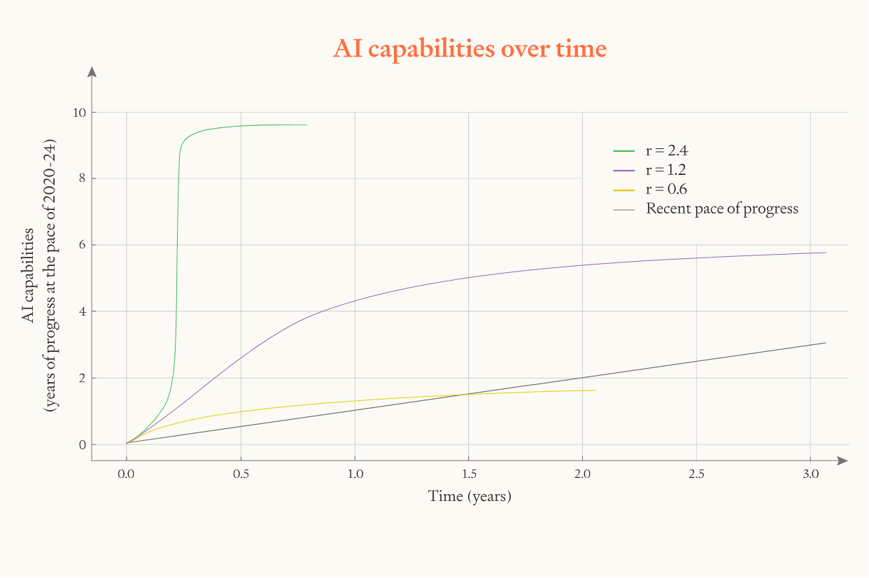
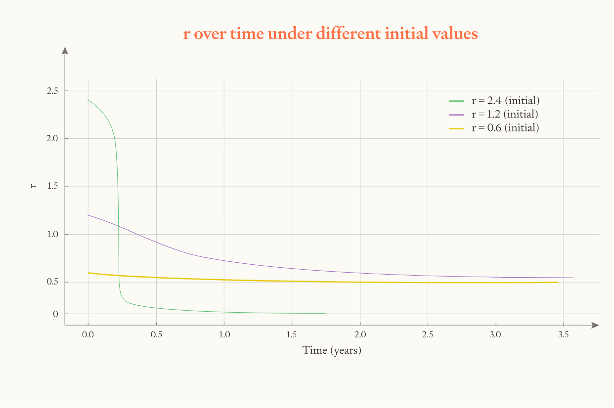
Once falls below 1, progress starts slowing. When is higher, software progress accelerates more quickly and it accelerates for longer (because software advances further before falls below 1).
Also, when starts higher, effective limits are approached more rapidly and so itself falls more rapidly.
Distance to the effective limits to software
We estimate that, when we train ASARA, software will be 6-16 OOMs from effective limits. This is equivalent to 6-16 years worth of AI progress (at recent rates) before capping out.
Software cannot keep improving forever. It will never be possible to get the cognitive performance of a top human expert using the computational power of a basic calculator. Eventually we hit what we will refer to as the “effective limits” of software.
How big is the gap between the software we’ll have when we develop ASARA and these effective limits? We'll focus on training efficiency. First we'll estimate how much more efficient human learning might be than ASARA’s training. Then we'll estimate how far human learning might be from effective limits.
Gap from ASARA to human learning
Human lifetime learning is estimated to take 1e24 FLOP.[15] As a very toy calculation, let’s assume that ASARA is trained with 1e28 FLOP[16] and that at runtime it matches a human expert on a per compute basis.[17] This means ASARA is 4 OOMs less training efficient than human lifetime learning.
There’s a lot of uncertainty here from the training FLOP for ASARA and the compute used by the human brain, so let’s say ASARA’s training is 2-6 OOMs less efficient than human lifetime learning.[18]
Gap from human learning to effective limits
But human lifetime learning is not at the limit of learning efficiency. There is room for significant improvement to the data used to train the brain, and to the brain’s learning algorithm.
Improvements to the data used in human learning:
- Not enough data – the brain is severely “undertrained”. Chinchilla optimal scaling suggests that models should be trained on ~20X as many tokens as they have parameters. On this account, the human brain is severely “undertrained”: it has maybe ~1e14 “parameters” (synapses) but only processes ~1e9 “data points” (1 data point per second for 30 years) during lifetime learning. If the Chinchilla scaling laws applied to the brain, then you could train a model with the same performance as the brain but with 4-5 OOMs less training compute – see this appendix. Of course, the brain architecture might have a completely different optimal scaling to Chinchilla. But it is very plausible that the brain is significantly undertrained due to hard biological constraints: organisms don’t live long enough to keep learning for 1000s of years! We'll call this 10-100,000X.
- Low fraction of data is relevant. Take a human ML expert. They only spend a small fraction of their time doing focussed learning that is relevant to doing AI R&D (at most 8 hours a day on average, and plausibly much less given the time spent on poetry, history, etc). This seems like a factor of at least 3-10X.[19]
- Data quality could be much higher. Even when humans are learning relevant material, the quality of the data they would be processing is far from optimal. When an outstanding communicator puts significant effort into organising and presenting content, human learning can be much more efficient. During the software intelligence explosion AI could curate better data sets still, including demonstrations of significantly superhuman performance. It seems like this would be at least 3X and plausibly 300X.
Improvements to the brain algorithm:
- Brain algorithms must satisfy physical constraints.
- Firstly, the human brain is spread out over three dimensions, communications from one part of the brain to the other must physically ‘travel’ this distance, and the speed of communication is fairly slow. This constrains the design space of brain algorithms.
- Secondly, the brain cannot do weight sharing (where the same numerical ‘weights’ are used in different parts of the network), which is essential to transformers.
- Thirdly, synaptic updates are local, just depending on nearby synapses, whereas AI can implement non-local learning rules like stochastic gradient descent where updates are instantaneously propagated throughout the entire network.
- AI algorithms will relax these constraints. On the other hand, the hardware first used to train AGI will have different constraints – e.g. around memory access. Also, evolution coevolved the brain’s hardware and software, which won’t be possible during a software intelligence explosion.
- It’s hard to know how significant this will be overall, maybe 3-100X.
- Significant variation between humans. There is significant variation in cognitive abilities between different humans. It may be possible to significantly increase human intelligence (e.g. by >100 IQ points) just by combining together all the best mutations and making more of the same kinds of changes that drive human variation. This might be another 3-10X.[20]
- Fundamental improvements in the brain’s learning algorithm. Evolution is a blind search process and does not always find the optimal solutions to problems – e.g. giraffes have a nerve that loops up and down their neck only to end up right next to where it started. AI could write vastly more complicated learning algorithms than the human brain algorithm, which is encoded within the human genome and so cannot exceed ~1e9 bits. In the limit, AI could hard-code knowledge GOFAI-style rather than learning it. Again, it’s hard to know how big this will be. Maybe 3-30X.
- Coordination. Humans must coordinate via language, which is slow and imperfect. By contrast, AIs could potentially communicate via multidimensional vectors and copies could share their activations with one another. This might significantly raise the collective capabilities achievable by large teams. Maybe 3-10X.
Overall, the additional learning efficiency gains from these sources suggest that effective limits are 4 - 14 OOMs above the human brain. The high end seems extremely high, and we think there’s some risk of double counting some of the gains here in the different buckets, so we will bring down our high end to 10 OOMs. We’re interpreting these OOMs as up limits upwards (increasing capabilities with fixed training compute) not as the limits downwards (reducing training compute but holding capabilities constant).[21]
So ASARA has room for 2 - 6 OOMs of training efficiency improvements before reaching the efficiency of the human lifetime learning, and a further 4 - 10 OOMs before reaching effective limits, for a total of 6 - 16 OOMs.
One reason for scepticism here is that these gains in training efficiency would be much bigger than anything we’ve seen historically. Epoch reports the training efficiency for GPT-2 increasing by 2 OOMs in a three year period, but doesn't find examples of much bigger gains over any time period. On the other hand, some of the factors listed are plausibly even bigger than our upper estimate, e.g. “must satisfy physical constraints” and "fundamental improvements”.
In recent years, effective training compute has risen by about 10X per year. So the model makes the assumption that after ASARA there could be 6 - 16 years of AI progress, at the rate of progress seen in recent years, before software hits effective limits.
To visualise how this parameter affects the results, we can run simulations with different limits.
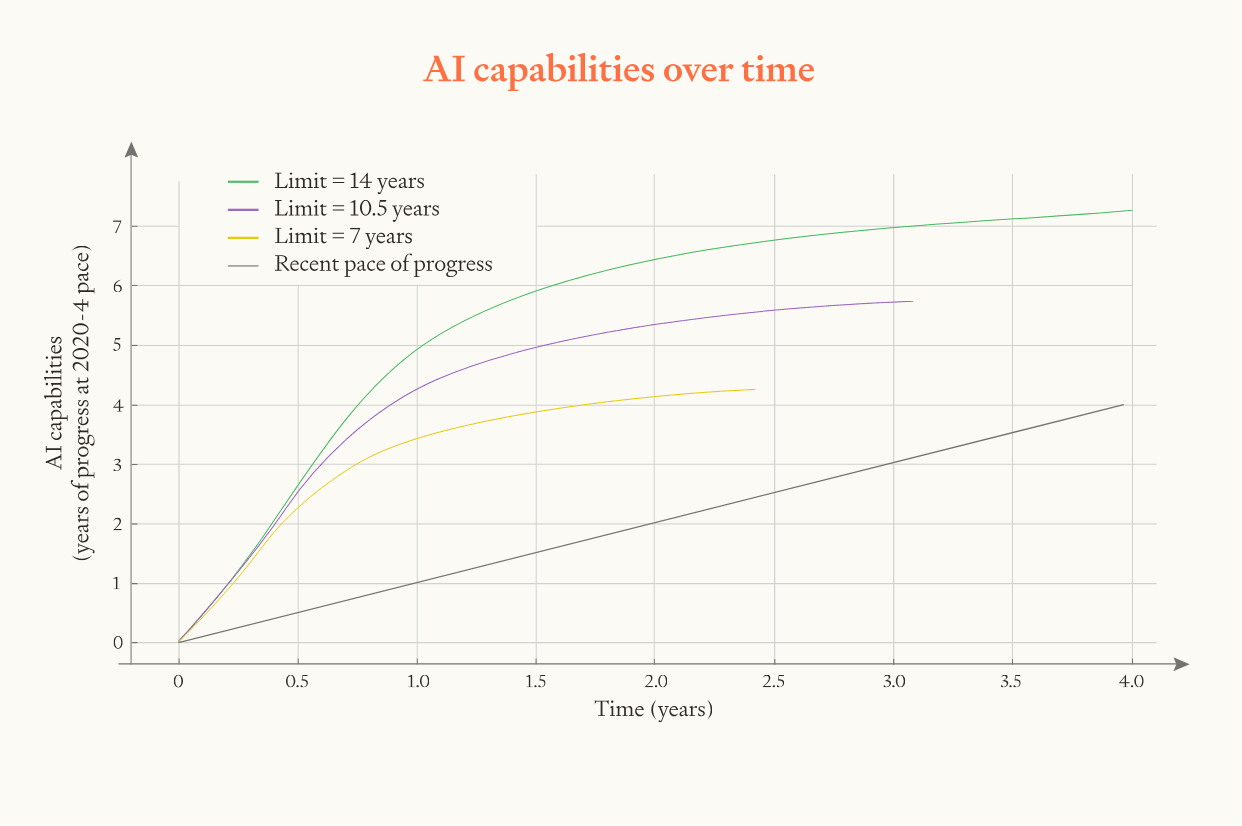
When effective limits are further away, software progress accelerates for longer and plateaus at a higher level.
Diminishing returns to parallel labour
Whether AI progress accelerates vs decelerates depends on the parameter . But how quickly it accelerates/decelerates also depends on another parameter, the diminishing returns to parallel labour .
The meaning of is: if you instantaneously doubled the amount of parallel cognitive labour directed towards software R&D, how many times would the pace of software progress double?
As discussed above, .
- captures diminishing returns to parallel efforts – nine women can’t make a baby in a month! We use .[22]
- captures the relative importance of cognitive labour inputs to software R&D, as contrasted with inputs of compute for experiments. We assume the share of software progress that’s attributable to cognitive labour is 0.5.
So our median estimate is .
We use a log-uniform distribution over from 0.15 to 0.6.
Summary of parameter assumptions
The Monte Carlo samples four parameters from, three from log-uniform distributions and one from a uniform distribution (distance to effective limits).
| Lower bound | Median | Upper bound | |
| Initial speed-up in the pace of software progress due to ASARA | 2 | 8 | 32 |
| Returns to software R&D, r | 0.4 | 1.2 | 3.6 |
| Distance to effective limits on software (in units of years of progress) | 6 | 11 | 16 |
| Diminishing returns to parallel labour, p | 0.15 | 0.3 | 0.6 |
Recall we derive our model from the following law of motion: We define p = λα and r = λα/β. Our median estimates of p and r correspond to α = 0.5, λ = 0.6, β = 0.25. Note that we independently sample p and r; we don’t sample the underlying λ, α, and β – we discuss this choice in an appendix. |
Box 2: What do our assumptions imply about the values of , α, and β?
You can change all of these assumptions in the online tool.
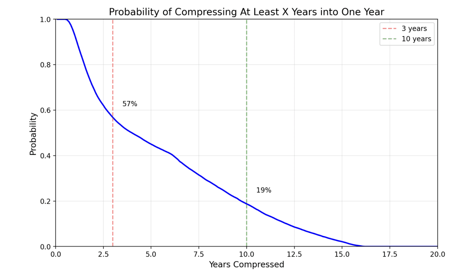
Results
| Years of progress | Compressed into ≤1 year | Compressed into ≤4 months |
| ≥3 years | 57% | 41% |
| ≥10 years | 18% | 12% |
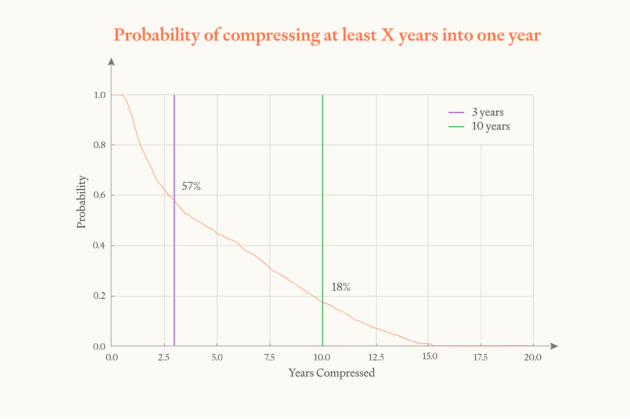
It goes without saying that this is all very rough and at most one significant figure should be taken seriously.
The appendix contains the results for two variants of the model:
- Retraining cost. This variant models the fact that we’ll need to train new generations of AI from scratch during the intelligence explosion and, if progress is accelerating, those training runs will have to become quicker over time. More.
- Gradual boost. This variant models AI systems intermediate between today’s AI and ASARA. It assumes AI gradually accelerates software progress more and more over time. More.
Both variants are consistent with the bottom line that the software intelligence explosion will probably compress >3 years of AI progress into 1 year, but is somewhat unlikely to compress >10 years into 1 year.
You can choose your own inputs to the model here.
Limitations and caveats
We're not modelling the actual mechanics of the software intelligence explosion. For example, there’s no gears-level modelling of how synthetic data generation[23] might work or what specific processes might drive very rapid progress. We don’t even separate out post-training from pre-training improvements, or capability gains from inference gains. Instead we attempt to do a high-level extrapolation from the patterns in inputs and outputs to AI software R&D, considered holistically. As far as we can tell, this doesn’t bias the results in a particular direction, but the exercise is very speculative and uncertain.
Similarly, we don’t model specific AI capabilities but instead represent AI capabilities as an abstract scalar, corresponding to how capable they are at AI R&D.
Significant low-hanging fruit may be plucked before ASARA. If ASARA is good enough to speed up software progress by 30X, earlier systems may already have sped it up by 10X. By the time ASARA is developed, the earlier systems would have plucked the low-hanging fruit for improving software. Software would be closer to effective limits and returns to software R&D would be lower (lower ). So the simulation will overestimate the size of the software intelligence explosion.
How could we do better? The gradual boost model variant does just this by modelling the gradual development of ASARA over time and modelling the software progress that happens before ASARA is developed. Our high-level bottom line holds true: the software intelligence explosion will probably compress 3 years of AI progress into 1 year, but is somewhat unlikely to compress 10 years into 1 year.
Assuming the historical scaling of capabilities with compute continues. We implicitly assume that, during the software intelligence explosion, doubling the effective compute used to develop AI continues to improve capabilities as much as it has done historically. This is arguably an aggressive assumption, as it may be necessary to spend significant compute on generating high-quality data (which wasn’t needed historically). This could also be conservative if we find new architectures or algorithms with more favourable scaling properties than historical scaling.
- We make this assumption when estimating the returns to software R&D , in particular when assessing the benefits of training models with better capabilities.
“Garbage in, garbage out”. We’ve done our best to estimate the model parameters fairly, but there are massive uncertainties in all of them. This flows right through to the results. The assumption about effective limits is especially worth calling out in this regard.
- You can choose your own inputs here!
Thanks to Ryan Greenblatt, Eli Lifland, Max Daniel, Raymond Douglas, Ashwin Acharya, Owen Cotton-Barratt, Max Dalton, William MacAskill, Fin Moorhouse, Ben Todd, Lizka Vaintrob and others for review and feedback. Thanks especially to Rose Hadshar for help with the writing.
Appendices
Derivation of our pseudo code from the semi-endogenous growth model
We start with the following environment (described in the main text):
Combining these three expressions we get the growth rate of software, as a function of software level and compute:
From here, the time it takes for software to double is given by
Next, if we want to express the doubling time under software level in terms of the doubling time for software under software level , we can divide expressions:
So we can see that after a doubling of software, the time it takes to complete the next doubling halves times. To map this expression to the parameters in the rest of this analysis, we define and as in the main text:
And therefore, to get the doubling time expression in the pseudo code note , therefore
Therefore, so long as we know the initial doubling time of software and and for each time period, we can chain together doubling times to calculate a path of software.
Additional model assumptions
In addition to the pseudo code, the results reported in the piece are also determined by three additional assumptions:
- AI software has recently been doubling every 3 months (more).
- Half of AI progress is due to software and half is due to compute (more).
- Our sampling procedure for the Monte Carlo (more).
AI software has recently been doubling every 3 months
A model parameter specifies the initial speed-up in software progress from deploying ASARA. But we also need to make an assumption about how fast AI software has progressed recently. Then we can calculate:
We assume that recently software has doubled every 3 months.
Why 3 months? Epoch estimates that training efficiency doubles every 8 or 9 months, but that doesn't include post-training enhancements which would make things faster. So we adjust down to 6 months. This is the doubling time of training efficiency – the training compute needed to achieve some capability level.
But the simulation measures “software” in units of parallel labour. A doubling of software is any software improvement as useful as an improvement that doubles the number of parallel copies you can run.
The main body argues that, measured in these units, software doubles more quickly than training efficiency because better training efficiency allows you to access better capabilities, and this is more valuable than having twice as many parallel copies. Based on this consideration, we adjust the 6 months down to 3 months.
Calculating the summary statistics
The simulation spits out a trajectory for AI software progress over time. From that we can calculate “there was a 1 year period where we had 10 years of software progress at recent rates of progress”.
But our results report how many years of overall AI progress we get in each year. So we must make an additional assumption about how the recent pace of software progress compares to the recent rate of overall AI progress. We assume that half of recent progress has been driven by compute and the other half by software.
To illustrate this assumption, it allows the following inference:
There was a 1 year period where we had 10 years of software progress → There was a 1 year period where we had 5 years of overall AI progress.
You can change this assumption in the online tool.
Objection to our sampling procedure
It might seem ill-advised to independently sample and . Should we not instead sample and ? After all, these are the more fundamental inputs that determine the model behaviour. For example, we will sample holding fixed – this means that a higher value for will change the (implicit) value of .
We tentatively think our sampling procedure is appropriate given our epistemic position. The best evidence we have to calibrate the model is evidence about . This comes from observing the ratio between the growth rate of inputs and the growth rate of outputs to AI R&D: . Given our evidence on , it is the case that from our epistemic position it is appropriate that a higher estimate of should change our estimate of .
To be concrete, suppose our evidence tells us that . Then we sample from our distribution over . If we sample a high value, it is appropriate for us to assume that is also high, so that our assumption about remains consistent with our evidence about .
A more sophisticated approach here is surely possible. But our model is intended as a glorified BOTEC and we don’t expect additional sophistication would significantly affect the bottom line. And our remaining uncertainty about the bottom line stems much more from uncertainty about the right parameter values than from uncertainty about the sampling procedure.
Variants of the model
We explore two variants of the model that make it more realistic in certain respects.
Retraining time
We have accounted for the time to train new AI systems in our estimate of the initial speed of software progress. But retraining also affects how the pace of AI progress should change over time.
Let’s say that AI progress requires two steps: improving software and retraining.
As software progress becomes very fast, retraining will become a bottleneck. To avoid this, some of your software improvements can be “spent” on reducing the duration of training rather than on improving capabilities. As a result of this expenditure, the pace of AI progress accelerates more slowly. (An inverse argument shows that the pace of AI progress also decelerates more slowly, as you can expand the time for training as progress slows.)
A simple way to model this is to assume that each time the pace of software progress doubles, the duration of training must halve. Software progress and training become faster in tandem.
How can we incorporate this into the model? Suppose that the model previously stated that software doubled times before the pace of software progress doubled. We should increase this to . The extra software doubling is spent on reducing the duration of training. Our rough median estimate for is 5, as argued in this appendix.
Specifically, we adjust the line of code that describes how software progress changes each time software doubles:
The exponent on 2 here is the reciprocal of . So we replace this exponent with
This analysis assumed that software was accelerating over time – , . Repeating the argument for the case where software is decelerating – , – yields . Therefore the correct exponent in both cases is .
We rerun the analysis with this new exponent and find that the results do not change significantly.
| Years of progress | Compressed into ≤1 year | Compressed into ≤4 months | ||
| RT | No RT | RT | No RT | |
| ≥3 years | 57% | 56% | 41% | 41% |
| ≥10 years | 19% | 17% | 14% | 12% |
See here for more analysis of how retraining affects the dynamics of the software intelligence explosion.
Gradual boost (from pre-ASARA systems)
In the main results we assume ASARA boosts the pace of software progress by 2-32x (median 8x) and the simulation starts from when this boost is first felt. In the ‘compute growth’ scenario we assume that this boost ‘ramps up’ (exponentially) over 5 years, mapping to the time frame over which we expect compute for AI development could continue to grow rapidly.
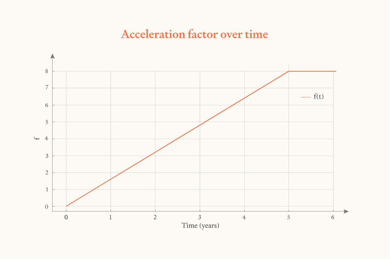
In the simulation, the initial boost to research productivity from deployment of AI is an additional 10% on top of the usual rate of software progress. The boost then grows linearly over time until it reaches the sampled maximum value (between 2 and 32).
To implement this in the model, we assume that the boost in each time period originates from compute growth, which grows at an exogenous (and exponential) rate until it reaches a ceiling. We assume this ceiling occurs after 12 doublings of compute (or a 4096× increase relative to the initial compute level) which occurs after five years from the start time of the model.
In the simulation it is assumed that . Given exponential growth in compute, increases linearly with time until it reaches the compute ceiling, at which point f remains at .
When running this version of the simulation we increase . This is because we previously discounted on account of software progress made in the run-up to ASARA making returns to software R&D more steep. But this simulation models the gradual ramp up to ASARA so this discount isn’t needed.
| Lower bound | Median | Upper bound | |
| r in other sims | 0.4 | 1.2 | 3.6 |
| r in this sim | 1.7/3 = 0.57 | 1.7 | 1.7*3 = 5.1 |
We also increase the distance to effective limits. The simulation starts at an earlier point in time when software is less advanced and further from limits. Epoch estimates that training efficiency increases by about 0.5 OOMs/year and, to include some intermediate speed up in software progress, we add 3 OOMs.
| Lower bound | Median | Upper bound | |
| Distance to effective limits in other sims | 6 | 11 | 16 |
| Distance to effective limits in this sim | 9 | 14 | 19 |
Here are the results:
| Years of progress | Compressed into ≤1 year | Compressed into ≤4 months | ||
| GB | No GB | GB | No GB | |
| ≥3 years | 59% | 56% | 48% | 41% |
| ≥10 years | 32% | 17% | 24% | 12% |
The software intelligence explosion is more dramatic, presumably because we used more aggressive parameter values for and the distance to effective limits.
Returns to software R&D: efficiency improvements only
In the main text, we include both runtime efficiency and capabilities improvements in our estimates of for software progress. But the capabilities improvements are necessarily more speculative: to pin down what counts as a doubling, we need to implicitly translate capabilities improvements into equivalent improvements in runtime efficiency.
To check how robust our main estimate is to this speculative translation, we can ask what is when considering only direct runtime efficiency improvements.
As above, the highest quality and most relevant estimate is Epoch’s analysis of computer vision training efficiency.[24] They estimate (every time the researcher population doubled, training efficiency doubled 1.4x).
Again we'll make a couple of adjustments:
- Downwards for runtime efficiency . To estimate returns to software improvements, we need to convert from training efficiency (the inputs) into runtime efficiency (the outputs). The logic of the Chinchilla paper implies that increasing training efficiency by 4X will increase runtime efficiency by between 2X and 4X.[25] This means we should reduce our estimate of by up to a factor of 2. We'll reduce it to .
- Upwards for post-training enhancements. Improvements to pre-training algorithms are not the only source of runtime efficiency gains. There are also techniques like: model distillation; calling smaller models for easier tasks; pruning (removing parameters from a trained model); post-training quantisation (reducing the numerical precision of the weights); more efficient caching of results and activations (especially for agents that re-read the same context multiple times). We'll increase our estimate to .
is necessarily lower when we’re considering only efficiency improvements - but it still seems fairly likely that , even excluding capabilities improvements.
Distance to effective limits: human learning
How much more efficient could human learning be if the brain wasn’t undertrained?
[Thanks to Marius Hobbhahn and Daniel Kokotajlo for help with this diagram.]
It looks like the efficiency gain is over 5 OOMs. Tamay Besiroglu wrote code to calculate this properly, and found that the efficiency gain was 4.5 OOMs.
Discussion of model assumptions
How the returns to software R&D r changes over time
Each time software doubles, decreases by a constant absolute amount; reaches 0 once software hits the ceiling.
The returns to software R&D are represented by the parameter . How does change over time?
One way to think about is: each time you double cumulative cognitive inputs to software R&D, software doubles r times.[26]
This means that if halves, the pace of software progress halves (holding the growth of cumulative inputs fixed). is directly proportional to the pace of progress (holding the growth of cumulative inputs fixed).
The model assumes that:
- By the time software reaches effective limits, . This means that further software progress is impossible.
- Each time software doubles, decreases by a constant absolute amount. This absolute amount is chosen to be consistent with #1.
- So, for example: once software has advanced half the distance to effective limits in log-space, the value of will have halved. Each doubling of cumulative inputs will double software half as many times as before.
This assumption could easily be very wrong in either direction. Returns might become steeper much more quickly, far from effective limits, perhaps because many OOMs of improvement require massive computational experiments that are not available. Alternatively, it’s possible that returns stay similar to their current value until we are within an OOM of effective limits.
How the speed of software progress changes over time
The math of the model states that every time software doubles, the pace of software progress doubles times.
Let’s assume software progress becomes faster over time (). How quickly does it become faster?
Let’s assume (which is close to our median conditioning on ) and , each time software doubles the pace of software progress doubles 0.18 times. In other words, a very rough median estimate is that, in a software intelligence explosion, every time software doubles 5 times, the pace of software progress itself will double.
This was created by Forethought. See our website for more research.
- ^
Greenblatt guesses that the improvement in capability from 6 OOMs of effective compute would be the same as 8 OOMs of rank improvement within a profession. We’ll take the relevant profession to be technical employees of frontier AI companies and assume the median such expert is the 1000th best worldwide. So 8 OOMs of improvement would be 8/3 = 2.7 steps the same size as from a median expert to a top expert.
- ^
Minor caveat: The starting point in this example (“30,000 top-expert-level AIs thinking 30x human speed”) corresponds to a slightly higher capability level than our definition of ASARA. We define ASARA as AI that can replace every employee with 30x copies running at 30x speed; if there are 1000 employees this yields 30,000 AI thinking 30x human whose average capability matches the average capability of the human researchers. Rather than top-expert-level ASARA is mean-expert-level.
- ^
AI-2027 median forecast is 8 months from the superhuman coder to the superintelligent AI researcher (SIAR). The superhuman coder roughly corresponds to ASARA (it’s better at coding and maybe a bit worse at ideation), so AI-2027 forecasts ~8 months from ASARA to SIAR. I estimate that SIAR is roughly 6 years worth of AI progress above ASARA. (Explaining this estimate: The gap between the SIAR and a top human expert is defined as 2X the gap between a top human expert and a median human expert within an AGI company. That latter gap corresponds to a 1000-fold rank ordering improvement (as the median lab expert is ~1000th best in the world). So SIAR is a 1 million-fold rank ordering improvement on the top human expert. The top human expert is maybe ~100-fold rank ordering improvement on top of ASARA, which matches the mean company employee and so is better than the median. So SIAR is maybe a ~100 million-fold rank ordering improvement on ASARA. Ryan Greenblatt estimates that a 100 million-fold rank ordering corresponds to 6 OOMs of effective compute, which is roughly 6 years of recent AI progress. So, SIAR is ~6 years of AI progress above ASARA. Of course, this is all very rough!) This means that AI-2027 forecasts 6 years of AI progress in 8 months. This is more aggressive than our median forecast, but not in the tails. AI-2027 then additionally assumes that very rapid AI progress continues so that after 5 further months AI is superintelligent in every cognitive domain (rather than just AI research, as for SIAR). If this is another 4 years of progress (at recent rates) then AI-2027 are forecasting 10 years of AI progress in 13 months, which corresponds to our ~20th percentile most aggressive scenarios. So, very roughly and tentatively, it looks like our model assigns ~20% probability to the software intelligence explosion being faster than AI-2027’s median forecast.
- ^
Note that Aghion, Jones and Jones (2019) describe a slightly different condition for infinite technological progress in finite time: . Our finite time explosion condition is slightly different due to the fact that in our model software levels enter the research inputs function. Explosion conditions for a similar model are presented in Davidson et al. (2025).
- ^
In the section below where we estimate the distance to effective limits, we first estimate this in units of ‘years of AI progress at recent rates’. We convert this to Doublings-Till-Ceiling by assuming AI progress has made 4 doublings of effective compute inputs per year.
- ^
There’s a spectrum of ASARA definitions that we could use, ranging from weak (e.g. a 10X increase in the cognitive labour going into AI R&D) to strong (e.g. a 100,000X increase). As AI improves, we’ll pass through the full spectrum. Both extremes of the spectrum have downsides for our purposes in this forecast. If we use a weak definition, then we’ll forecast a software intelligence explosion that is initially slow and accelerates gradually over time, e.g. over multiple years, eventually still becoming very fast. But then we’ll miss the fact that rising compute (which we’re not modelling) will cause the software intelligence explosion to accelerate much more quickly than our forecasts. Alternatively, we could use a strong definition of ASARA. But then we’ll have only achieved ASARA by already making significant rapid software progress – i.e. a big chunk of the software intelligence explosion will have already occurred. Our definition attempts to balance these concerns. A variant of this model discussed below considers ASARA being gradually developed, which avoids the need to choose one arbitrary point in the sand.
- ^
Of course, in fact ASARA will have very different comparative strengths and weaknesses to human researchers. We can define ASARA as AI which is as impactful on the pace of AI progress as if it replaced each human with 30 copies each thinking 30X faster.
- ^
They happen to calculate the speed-up from exactly the definition of ASARA we are using here: replacing each researcher with 30X copies each thinking 30X as fast.
- ^
In areas of technology, if you double your research workforce overnight, the level of technology won’t immediately double. So we look at how many times output (in this case, efficiency) doubles when the cumulative research inputs doubles. On this definition of ‘cumulative input’, having 200 people work for a year constitutes twice as much cumulative input as having 100 people work for a year.
- ^
What does it mean for software to “double”? See box 1 a few paragraphs below!
- ^
Epoch’s preliminary analysis indicates that the value for LLMs would likely be somewhat higher. We don’t adjust upwards this, because it’s a speculative and probably minor adjustment.
- ^
You get the answer to this question by taking these estimates of and then adding 0.5. Why? Doubling training efficiency has two effects:
- First, you can train a model with 2X the effective compute (your compute is the same, but you’ve doubled training efficiency, so effective compute is doubled too). This doubles your output-per-runtime-FLOP times, as estimated in the source. This effect is equivalent to doubling runtime efficiency times.
- Secondly, it also allows you to run that model with sqrt(2) less compute. This literally doubles runtime efficiency 0.5 times.
- So if you double training efficiency this increases output by the same as if you’d doubled runtime efficiency times.
- ^
This isn’t actually a fixed hardware scale, because the hardware required decreases over time. A fixed hardware scale might see slightly faster improvements.
- ^
See Nagy et al (2013) and Bloom et al (2020).
- ^
This assumes the human brain does the equivalent of 1e15 FLOP/second and lifetime learning lasts for 30 years (=1e9 seconds).
- ^
This is 10X less than Epoch’s estimate of what the biggest AI lab could achieve by the end of the decade
- ^
In other words, each FLOP of computation is (on average) equally useful for doing AI R&D whether it’s done by ASARA or done in a human expert’s brain. Why make this assumption? It matches our definition as ASARA as AI that increases cognitive output for AI R&D by ~1000X. If the lab uses the same amount of compute for training ASARA as for running it (1e21 FLOP/s), and ASARA matches humans on a per-compute basis, and the human brain uses 1e15 FLOP, then the lab could run 1 million human-equivalents. If there are 1000 human researchers then they could run 30 copies of each thinking 30X as quick, matching our definition of ASARA. See calc.
- ^
Thanks to Carl Shulman for this argument.
- ^
3X relative to humans spending 8 hours a day on focussed learning, as AI systems could do this for 24 hours a day.
- ^
A rough BOTEC suggests that using 2X the computation in human lifetime learning corresponds to ~30 IQ points, so 100 IQ points would be 10X.
- ^
We think the downwards limits could be much smaller as, expanding downwards, you eventually hit very hard limits – it’s just not possible to train AGI with the amount of compute used in one GPT-4 forward pass.
- ^
We're not aware of good evidence about the value of this parameter. See discussion of this parameter here under “R&D parallelization penalty”.
- ^
In this model, synthetic data generation probably should be considered a technique to increase effective training compute – get better capabilities with a fixed supply of compute.
- ^
Epoch also analysed runtime efficiency in other domains:
- Computer chess:
- Boolean satisfiability:
- Problem solvers:
- Linear programming:
These estimates are broadly consistent with our median estimate above of .
- ^
If we assume all efficiency improvements come from making models smaller (i.e. achieving the same performance with fewer parameters), then we’d expect training efficiency to grow twice as quickly as runtime efficiency. This conclusion is implied by a landmark 2022 paper from DeepMind, often informally referred to as the “Chinchilla paper.” The Chinchilla paper found that when training an LLM with a fixed computational budget, it’s best to scale the size of the model and the amount of data used to train the model equally; therefore, if a model can be made times smaller, the runtime efficiency will grow by , while the training efficiency would grow by (since training on each data point will require as much computations, and you will only need to train on as many data points as well). This line of reasoning, however, does not apply to efficiency improvements coming from other avenues, which in many instances will have comparable effects in speeding up training and running systems.
- ^
“Inputs” as defined here do not account for stepping on toes effects: having twice as many people work for the same amount of time produces twice as much input.
OscarD🔸 @ 2025-08-05T18:17 (+4)
a major paradigm shift that enables massive progress without significant increases in effective compute
I am confused here - I thought by definition if capabilities have gone up, that is an increase in effective compute? As to estimate effective compute we just ask how much more compute would you need to use in the old paradigm to get the same performance. Maybe you mean the answer is 'infinity' as in no amount of compute in the old paradigm would get performance as good as after the paradigm shift?
Tom_Davidson @ 2025-08-11T16:44 (+4)
Thanks, good Q.
I'm saying that if there is such a new paradigm then we could have >10 years worth of AI progress at rates of 2020-5, and >10 OOMs of effective compute growth according to the old paradigm. But that, perhaps, within the new paradigm these gains are achieved while the efficiency of AI algs only increases slightly. E.g. a new paradigm where each doubling of compute increases capabilities as much as 1000X does today. Then, measured within the new paradigm, the algorithmic progress might seem like just a couple of OOMs so 'effective compute' isn't rising fast, but relative to the old paradigm progress (and effective compute growth) is massive.
Fwiw, this X thread discusses the units I'm using for "year of Ai progress", and Eli Lifland gives a reasonable alternative. Either work as a way to understand the framework.