A Primer in Causal Inference: Animal Product Consumption as a Case Study

By Jared Winslow, MMathur🔸 @ 2025-04-16T14:28 (+28)

Introduction

This post explains some key causal inference concepts for nonrandomized longitudinal studies. With those principles in mind, we can weigh in on some recent results in animal advocacy.

Causal inference is a branch of statistics that addresses when, and how, we can arrive at causal conclusions when a treatment was not–or could not be–randomly assigned. As a case study, we’ll review the reanalysis of a recent study by Bryant Research, “A longitudinal study of meat reduction over time in the UK.” I led this reanalysis (along with Maya Mathur) within my role at the Humane and Sustainable Food Lab.

A notable strength of the original study was its large sample of 1,500 participants and year-long data collection across three separate waves. As we’ll see, well-designed studies with multiple waves of data collection can provide a compelling basis for causal inference^[1]. In fact, Bryant Research is one of the few to have collected such data on animal product consumption! 

However, limitations within their statistical modeling made it difficult to interpret the estimates as causal or as meaningful associations. We addressed these issues by using a standard causal inference modeling approach (published in Food Quality & Preference). 

To unpack the issues, let’s start with the fundamentals.

Causal inference: A Primer

It’s often said that establishing causality rests on three foundations–originally proposed by John Stuart Mill^[2]:

1. Co-occurrence:  Treatment and outcome occur together regularly and consistently.
2. Temporal precedence:  Treatment precedes outcome^[3].
3. No alternative explanations:  No hidden factors explain the observed relationship.

To disentangle these assumptions, let’s craft a fake example relevant to our problem of animal product consumption. Imagine that we collect a single wave of study data (i.e., a cross-section) and record participant habits related to diet. In our sample, we observe that some participants consume less animal products than others. Let’s say that these particular participants also self-report to both i) socializing with vegans and vegetarians and ii) being generally motivated to decrease their animal consumption.

With a single wave of data, we have enough information to justify the first assumption: co-occurrence. Assuming–because why not–that the study design and analysis are otherwise robust, we can infer that socializing with vegans seems related to the (perhaps) less frequent consumption of animals, but not much more than that. While much of modern statistics addresses association, it doesn’t get us far in answering causal questions–if one truly caused the other–without more assumptions. Was it that having vegan friends caused people to eat less meat, or simply that people who eat fewer animal products naturally get along with vegans? Without data from at least two separate time points, we have no way of ruling out reverse causation, and no way of knowing which caused which. 

To that end, let’s introduce a second wave to our imagined study, measuring socialization and motivation during the first wave and animal consumption during the second wave. By collecting measurements where the hypothesized cause is before the hypothesized effect, we can isolate a direction of influence and test it. (If we wanted to test whether animal consumption induces motivation and socialization, we would do the opposite.) With two waves, our resulting estimates should reflect something closer to the causal effects of socialization and motivation on consumption. Temporal precedence, resolved. There is a larger issue, though: we haven’t ruled out alternative explanations. What if internal motivation is what actually fuels the fire for both socialization and reducing animal consumption, and socialization doesn’t have any effect at all! And if that were the case, there should be no reason to think we can intervene on animal consumption through some form of socialization.

To better understand the ‘alternative explanations’ problem, let’s deconstruct it. In statistical jargon, this condition confusingly has fifty-some names: nonspuriousness, unconfoundedness, no omitted variable bias, exogeneity, backdoor criterion, exchangeability, ignorability of the treatment assignment^[4]. In principle, it’s simple: did you rule out confounding variables that would bias your estimated effect (e.g., causes behind both the treatment and the outcome)? For regression, one method would be to simply add the confounding variables to your set of predictors (called “controlling for confounders”)^[5], but in practice we often lack these confounders and are simply adjusting rather than fully controlling. In contrast, randomization inherently resolves confounding in expectation by ensuring the treatment and control groups are identical on average^[6].

You may be asking, why don't we just collect two waves, add first wave measures of socialization and motivation to our set of predictors, and task the model with adjusting for both? The need to control for confounders creates another problem, however, called overadjustment. That is, we want to control for confounders, but not for variables that are mediators (mechanisms by which the treatment affects the outcome). Controlling for mediators will generally bias our estimate.

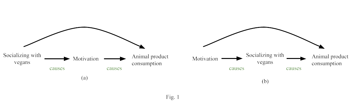
In the left diagram (Fig. 1 a), socializing is a confounder, and we must control for it to estimate the causal effect of motivation on animal product consumption. But in the right diagram (Fig. 1 b), socializing is a mediator, and we must not control for it to estimate the causal effect. Either way, to resolve this issue, we need a third wave of data collection occurring prior to the treatment. By measuring motivation at the earliest wave, we know it cannot be a mediator, and so we can control for it to reduce confounding and thereby get better estimates for the effect of socialization on consumption^[7]. Conversely, if we want to assess it as a treatment, we measure it at the second wave, or if we want to assess it as an outcome, we measure it at the third wave. 

Of course, since we can rarely control for all confounding variables, a central question is how robust our results are to plausible amounts of unmeasured confounding (given the variables we did manage to control). Sensitivity analyses–tests that assume different levels of unmeasured confounding–can help address this goal quantitatively, and help us better calibrate our confidence in different results.

A critical point to take from this is that satisfying all three assumptions (in general) necessitates at least three separate waves of data. With that in mind, let’s turn to the real data!

Original Analysis

Bryant and team had two primary outcomes: participant 1)  animal product consumption, and 2) six-stage ideation towards reducing meat / becoming vegetarian. For predictors, their survey covered a broad array of potential influences:

Behavioral Factors

• Capability [to reduce meat consumption]
• Opportunity
• Motivation

Social Interactions

• Killing animals
• Interacting with animals
• Socializing with vegetarians/vegans

Media Exposure 

• Online media [on the negative impacts of animal product consumption]
• Traditional media
• Outdoor media (billboards + activism)

Food Behaviors

• Handling raw meat
• Plant-based analog (alt protein) consumption

Vegan Challenges

• Veganuary
• Challenge 22+
• No Meat May
• Vegan Easy 30-Day Challenge

Each of these exposures were measured across all three waves.

Again, this design perked up our ears because having three waves of data made causal inference by confounder adjustment possible. The original analysis did not leverage the multiple waves and essentially treated the data as cross-sectional (all predictors were included in a single model for each outcome). There are two key statistical problems with this:

1. Post-treatment bias:  Including potential mediators (i.e., variables measured after the treatment) distorts the estimated effects.
2. Gain scores:  Outcomes were change scores – subtracting wave 1 from wave 3. In observational data, this approach can lead to substantial bias.

Ideally, we would regress the change score on predictors measured before or at the first time point (here, Wave 1 or earlier). When predictors are measured between rather than before the starting point of the change scores, the resulting estimates lack meaningful interpretation. This is because the outcome now contains information from Wave 1, and the potential treatment was measured after that. Even change score analyses done in the standard way generally do not estimate causal effects in nonrandomized studies. 

It’s often better to let the model adjust for predictors directly than to do so manually through differencing. Conditioning on the baseline (adding it as a predictor) adjusts for it—like subtracting it out, but in a way that better respects the structure of the data and the assumptions of the model.

Bryant et al.’s results counter-intuitively showed that motivation to reduce meat consumption and exposure to outdoor media addressing the negative impacts of eating animal products both correlated with increased actual animal product consumption. For motivation, an inverse relation! Also, killing animals was shown to be both negatively and positively related with animal product consumption, depending on which wave’s measure you looked at. Did these hold up to reanalysis?

Our Approach

To address the above limitations, we took a modular approach: a separate model for each predictor of interest, rather than a single centralized model. Each model ensured temporal ordering by separating variables by wave:

• Wave 1 variables: Confounders (plus demographics)
• Wave 2 variable: Exposure of interest
• Wave 3 variable: Outcome

Within an individual model, we focus on a single exposure / treatment of interest, and we use this variable measured at Wave 2 as the key predictor in the model to assess co-occurrence. We use the outcome measured at Wave 3 to ensure temporal precedence of the Wave 2 predictor. We then control for all variables measured at Wave 1 to reduce confounding in an attempt to rule out alternative explanations. Being Wave 1 measures, we know the controlled variables are not mediators. 

If we had three potential exposures of interest–Veganuary participation, interactions with activism (a subset of outdoor media), and plant-based analog (alt protein) consumption–we would have three models for a single outcome:

1. ${\text{outcome}}_3\sim {\text{veganuary}}_2+{\text{veganuary}}_1+{\text{activism}}_1+{\text{altprotein}}_1+{\text{outcome}}_1+\text{demographics}$
2. ${\text{outcome}}_3\sim {\text{activism}}_2+{\text{veganuary}}_1+{\text{activism}}_1+{\text{altprotein}}_1+{\text{outcome}}_1+\text{demographics}$
3. ${\text{outcome}}_3\sim {\text{altprotein}}_2+{\text{veganuary}}_1+{\text{activism}}_1+{\text{altprotein}}_1+{\text{outcome}}_1+\text{demographics}$

where the number suffixes refer to the wave of measurement.

In the first model, the single coefficient of interest is that of Veganuary 2, representing the association between Veganuary participation at Wave 2 and the outcome at Wave 3, holding constant all variables at Wave 1 and demographics. The association can be interpreted as a causal effect only if we have successfully controlled for all actual confounders (unlikely unless we can do so by design). For the actual reanalysis, this amounted to 30 different models. 

Results

Before peeking at the results, try guessing the strongest predictors without seeing the answers. Was it opportunity? Outdoor media? Online media?

Spoiler ahead!

Significant Predictors of Animal Product Consumption

• Outdoor media → +3 (more consumption!)^[8]
• Plant-based analog consumption → −3
• Motivation to reduce → −4

(The units are monthly consumption occurrences, so −3 means ~one full day's consumption less per month.)

The outdoor media result did hold up. Also, tying things back to our fake example, we have evidence for motivation's significance (in the opposite direction of Bryant et al.), but not for socialization's. 

Significant Predictors for Progression Toward Vegetarianism

• Handling raw meat → −0.05 (behavioral regression)
• Plant-based analog consumption → +0.12
• Motivation to reduce → +0.11
• No Meat May → +0.64
• Vegan Easy 30 → +1.4

(The units are a person's stage on a six-stage behavior/ideation scale from “completely uninterested” to “vegetarian for life”. A 1.4 increase is one stage and a half and is substantial.)

Now, do the estimates represent real causal effects? Well, not necessarily. While we did control for all available confounders, there could be influential confounders that went unmeasured. Most likely, our results are less biased than unadjusted estimates, but they probably still have some residual confounding bias. 

Furthermore, statistical significance does not imply practical significance. Although not statistically significant for animal product consumption, the largest effect sizes for that outcome were from vegan challenge participation. Estimates for all four vegan challenges were between -5 and -8 (roughly double that of plant-based analog consumption). The lack of statistical significance may be due to low power, given the very small proportion of challenge participants in the study. 

Takeaways

First, in line with intuition, motivation to reduce meat consumption was associated with subsequent reductions in animal product consumption. Again, this is contrary to the unexpected result found by Bryant et al that motivation to reduce meat consumption leads to increased actual consumption. Handling raw meat was associated with later increases in animal product consumption. While this may seem self-evident (eating meat requires cooking meat), we should remember this result is estimated after conditioning on prior animal product consumption and other variables, so it may reflect more than that.

More interestingly, exposure to activism (isolated from outdoor media) was indeed associated with increased animal product consumption. Future work should further investigate this finding on activism to see whether the result replicates, and if it does, to understand i) what constitutes “activism” in participants’ minds and ii) why certain messages or delivery may be backfiring.

The real leads we have are that both plant-based analog consumption and vegan challenge participation seem to reduce animal product consumption. The key question is how much of these effects could be due to unmeasured confounding that is not adequately captured by the measured variables. Sensitivity analyses indicated that a moderate (but not extreme) amount of unmeasured confounding would be needed to potentially overturn some of these results.

Some last limitations: There was nonresponse within waves, attrition across waves, and consumption patterns are self-reported. Hopefully, future work can measure consumption externally (e.g., with purchasing data). Being only a single study, we hope to see similar designs replicated. Nonetheless, we can learn a lot methodologically and substantively from this study.

Many thanks to Bryant Research for designing and conducting the study, and special thanks to Chris Bryant for being exceptionally supportive of our doing a reanalysis. This openness to collaboration makes finding clearer answers all the more possible.

1. ^{^}

   Other nonrandomized designs, such as quasi experiments, can also provide a strong basis for causal inference.

2. ^{^}

   Technically this isn’t actually true. Mill’s original five methods were neither necessary nor sufficient for establishing causality, and later work–done by many scientists–distilled his canons into three modern principles. These ideas trace back to David Hume and undoubtedly to many others.

3. ^{^}

   Cause and effect may be far apart in time and space yet still “occur together” according to a nonlinear relationship exhibiting zero Pearson correlation. Also, cause and effect may be embedded within a feedback loop where “cause precedes effect” but at a timescale that is difficult to determine.

4. ^{^}

   There are other, more technical assumptions—like no interference, consistency, and positivity – that serve to support the big three. These could be violated if, for example:

   1. Participants affect each others' outcomes.
   2. There are multiple "versions" of the treatment.
   3. The treated and untreated groups lack similarities.
5. ^{^}

   Other examples of causal identification strategies include regression discontinuity, instrumental variables, matching, and propensity score weighting. Causal identification means “having a strategy to make our causal assumptions hold.”

6. ^{^}

   Both on average and in expectation are necessary. On average says that, while there may be individual differences between the treatment and control groups, their respective means are the same. In expectation says that, over many randomizations, the respective means of all characteristics will converge, so confounding cancels out in the long run.

7. ^{^}

   We just need to remember that any resulting estimates attempt to capture average treatment effects. 

8. ^{^}

   Interestingly, if ‘outdoor media’ is separated into activism and billboards, both are still significant and reflect an increase in animal product consumption.